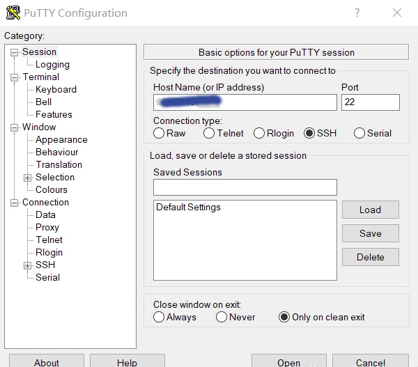
Managing Linux servers or Docker containers needs a basic understanding of the terminal, also known as the command line. Windows users, for example, can use the program PuTTY to obtain remote access via Secure Shell (SSH). The SSH is a secure remote connection that establishes an encrypted terminal connection to a Linux machine. SSH provides two basic types of access to a remote system. The not recommended way is via user /password or the better secure variant with a provided RSA encryption key pair.
Per definition, “terminal” and “shell” are not the same but are often used as synonyms. In general, is the terminal just the command line interface (CLI) that receives keystrokes from user interaction. The shell is an interpreter who runs inside the terminal to execute programs. For most Linux distributions, BASH (Bourne Again Shell) is the default system shell. Besides the BASH, there exist other shell variants like KornShell (ksh) or C Shell (csh).
When gaining access to a machine, whether through a reverse shell or SSH, the terminal may behave unusually. Common issues include the inability to clear text, use CTRL+C or CTRL+L, and improper text display. Here’s how to improve terminal navigation.
Steps for a Better Terminal Experience
1. Start a Temporary Script
script /dev/null -c bash
This starts a script that automatically deletes itself, as it points to /dev/null.
2. Send Reverse Shell to Background
Press CTRL+Z. This puts the reverse shell process in the background.
3. Resume the Process and Configure stty
stty raw -echo; fg
This returns you to the process and adjusts the terminal for rawer input and no echo.
4. Reset the Terminal
reset xterm
Use this command even if the text doesn’t display correctly or there are strange indents.
Replace [real console row number] and [real console column number] with the corresponding values found by running stty size in a normal console.
Security hint: Linux server machines that are reachable on the internet should not provide the login via superuser (root), neither as account password access. The problem we face is a distributed brute force attack from botnets to gain an administrative shell and hijack the system. Modern harden Linux servers disable the root account and just provide the sudo command for administrative users.
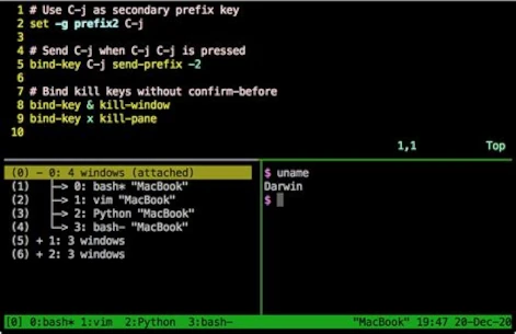
Administrators who need to deal with multiple open shells to maintain different machines like to use a very handy tool called TMUX [1]. Currently available in Version 3 and easily installed via shell.
apt-get install tmux
TMUX is a program that allows multiple terminal sessions in one terminal. For the correct usage, you should consult the official manual page [2]. The program is a bit complex to use and needs a little time to learn. A short workshop is too large for this post and would fit into its own article, may get published in the future. Just to give an idea of the possibilities they can do with TMUX check the following screenshot.
Developers with some networking experience know that a user’s IP address can reveal some interesting details. These details include information about the country and city of origin, as well as the internet service provider (ISP). This makes it possible to effectively identify and block the increasingly popular proxy servers. Of course, geolocation is just one piece of the puzzle in uniquely identifying users.
The current version of GeoIP is 2, which has completely replaced the outdated version 1. GeoIP2 is a service provided by MaxMind [1], which also offers a free community version. For example, if you run a self-hosted analytics tool like Matomo, you should ensure your web server is correctly configured for GeoIP2 to guarantee full functionality.
There are two ways to integrate GeoIP2 into your own server. Option 1 is the simpler option using a PHP module. Option 2 is more powerful but requires more server administration knowledge. In this solution, we use GeoIP2 as an Apache2 module.
Anyone who already has Fail2Ban [2] running correctly on their own server might be considering whether it makes sense to link Fail2Ban with GeoIP2. This is certainly possible, but it has more advantages than disadvantages, because Fail2Ban operates directly on the Apache log files. This is why Fail2Ban can only become active on the second request from an IP address. To activate GeoIP2 in Fail2Ban, a corresponding filter must be set, which can quickly have a negative impact on performance on servers with high user load. Therefore, it is better to monitor the requests to the server and block specific countries directly via the request in case of suspected attacks. However, this requires GeoIP2 to be installed and configured as an Apache module.
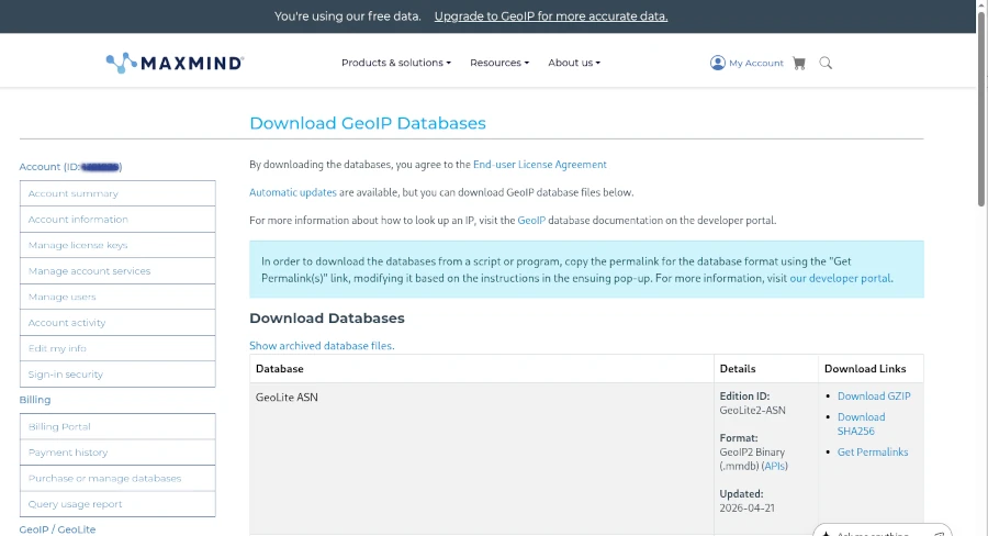
Before we can begin, however, we need to create a free account with MaxMind and download the free GeoIP2 (Lite version) databases for our example.
Once the first hurdle is cleared, we can get started. To use GeoIP2 in PHP applications, a suitable library is required. Using Composer as a dependency manager, the geoip2/geoip2 library can be included in its latest version.
As you can see, the directory for the MaxMind GeoLite database must also be specified during initialization. This option is particularly suitable for those using a managed server or web space who have no control over the installed environment. However, you should avoid using PECL (PHP Extension Community Library), as it has been marked as deprecated and will be replaced by PIE (PHP Installer for Extensions) [4].
Integrating GeoIP2 globally for all PHP applications requires a bit more effort. The basic requirement is a functioning Apache 2/PHP installation on a Linux operating system. If this is the case, only a few steps are necessary:
Install the maxminddb library
Download the PIE PHAR library
Install maxminddb for PIE and activate the extension in the php.ini file
Deploy the GeoLite databases on the server Before following this path, however, you should consider whether it would be better to deploy MaxMindDB as an Apache module. The most significant advantage of this approach is its high speed, which prevents the server from crashing even under heavy user load. The Apache module provides environment variables that can be used for filtering directly in the Apache configuration. The biggest challenge is compiling the Apache 2 module.
To keep this short workshop concise, I’ll demonstrate all the necessary steps in the php-apache:8.4 Docker container. Of course, it should be easy to adapt the corresponding commands slightly for a natively installed Apache HTTP Server.
In line 13, we copy the mod_maxminddb version 1.3.0, previously downloaded from GitHub [5], into the container to compile it in the next step. The important addition in line 16, which suppresses the error message that automake version 1.6 is required, is crucial. Afterward, the module can be activated, and the databases downloaded from MaxMind should also be copied into the Docker container. Finally, the module configuration for Apache in the geoip.conf file must be configured and activated. The content of the configuration file is as follows:
The firewall, or firewall, was always a spectacular event in the days of the circus and traveling performers. People or animals would leap through it and be cheered by the crowd. However dramatic such a performance may have seemed to the spectators, the spectacle was quite calculated for the acrobat. After all, we know that fire is one of the most powerful primal elements that humankind has tamed.
In cybersecurity, the firewall is one of the most fundamental protective mechanisms for networked computer systems. This applies to both home computers and mainframes in data centers. However, the idea of igniting one or more rings of fire around a computer is more comparable to a circus spectacle, often melodramatically depicted in movies. Statements like “The first firewall has fallen and the second is already 70% breached” are perfect for the screen but have nothing to do with reality.
Before we delve into the details, let’s briefly consider how computer systems are connected to form a network. The crucial detail we need is the IP address. In simpler terms, the IP address is the telephone number of the computer or device on the network. To connect to another computer, you need to know its IP address, just like a telephone and its phone number. Once the connection is established, information, or data, can be exchanged between the two devices. This information is broken down into small, manageable packets by the various internet protocols. A protocol is a defined set of rules that all participants must follow. This can easily be compared to sending a letter or package through the mail.
Write the letter.
Put the letter in an envelope and seal it.
Write the recipient’s address on the front of the envelope.
Write the sender’s address on the back of the envelope.
Attach a sufficient stamp to the envelope and drop it in the mailbox.
Write the letter.
Write a … Without knowing the internal workings of the postal service, we can assume that the letter will reach its recipient if we follow the protocol correctly. The same applies to the internet. Depending on the type of data, the computer selects a suitable program that implements the protocol for us. Based on the Internet Protocol (IP), which governs the connection between computers, there are other protocols that handle the data. Well-known protocols include HTTP(s) for websites and FTP for sending files.
Now let’s get to the main topic. What exactly is a firewall and what is it used for? Imagine a very long hallway with countless doors—65,536 doors to be precise. These doors can be opened inwards or outwards. We can therefore move from the hallway to the outside (outgoing traffic) or from the outside into the hallway (incoming traffic).
A Browser Game, (c) mediasinres.tv
These doors are called ports in technical jargon, and they have a fixed number. If you install special programs on your computer that can communicate with other computers, these programs are usually bound to such a port. Here’s a small example: Long before WhatsApp and similar apps, there was Internet Relay Chat, or IRC for short. If you installed IRC on your computer, it was hidden behind port 194. An important characteristic of ports is that if a program is already bound to a port, no other program can use that port.
A firewall allows you to selectively block these gateways to and from the internet. Basically, there are four different options for each gateway:
Completely blocked,
Inbound blocked,
Outbound blocked, and
Completely open.
Let’s return to our IRC example. If the gateway is completely blocked, we cannot send or receive messages, even though the program can be started on our computer. It cannot establish a connection to the network. If the inbound gateway is blocked, we cannot receive messages, but we can send them. If the outbound gateway is blocked, we can receive messages, but we cannot send any ourselves.
The biggest problem with using firewalls is that they are often not configured correctly. We distinguish between two options here. The most common option is called a blacklist and only regulates the ports specified in the list. Considering that there are 65,536 ports, this can become a very long and unwieldy list. The risk of forgetting something is very high. The advantage of this option is that it is very robust for inexperienced users. The other option is the so-called whitelist. This works in exactly the opposite way to the blacklist. By default, all ports are closed, and the user must explicitly specify which ports are allowed to be opened. As you can easily imagine, operating in whitelist mode requires a certain amount of user experience. You have to know which port belongs to which program and how to enter these rules into the firewall.
As we can see, the image of drawing a ring of fire around the computer is not a suitable way to visualize how a firewall works. Once the door—that is, on the computer—is blocked, installing another firewall on the computer makes little sense. In this case, the saying “two is better than one” doesn’t apply.
Attacks on firewalls typically involve searching for open ports and then exploiting them. This is done using so-called port scanners. Anyone wanting to try out such a port scanner shouldn’t do so without authorization. Searching for open ports on other people’s computers is already a criminal offense in Germany and many other parts of the world.
Another, very advanced attack scenario involves attacking the firewall program itself. Here, the aim is to find and exploit any existing programming errors in the firewall.
Firewalls are available for every operating system in a wide variety of forms. Professional network devices such as routers and switches may also have integrated firewalls. In this case, the router acts as a network computer and protects all devices connected to it. Before deciding on a specific program, you should find out that it is as easy to use as possible and comes from a reputable manufacturer.
List (incomplete) of the most well-known standard ports:
The permanent storage of data is called persistence in technical terms. To be able to access this data again, software is needed that structures and searches it. Such software is called a Database Management System (DBMS). To access a database from a programming language like Java, Ruby, Python, or PHP, a corresponding driver is required. This driver is often referred to as a client, because the DBMS is the server that allows access for multiple clients. In this article, we won’t focus on how to connect to the respective databases with which programming language, but rather on the different database technologies and their applications.
[Relational DB (rows, columns) | GIS DB | embedded DB]
[NoSQL | Key Value Store | Document DB (JSON, XML) | Graph DB | Time Series Server]
There are now numerous solutions to choose from for classic database systems, the so-called relational databases. Both commercial and professional free open-source options are vying for users’ attention. Most web hosting providers offer their users the choice between the free DBMS MySQL (Oracle) and MariaDB (a fork of MySQL after its acquisition by Oracle) for data storage. However, those who can manage their own servers can, of course, opt for the more professional PostgreSQL.
PostgreSQL is rather unsuitable for most standard PHP applications, although WordPress and Joomla do support this database system. Problems usually arise with the developers of extensions. Instead of using the application’s interfaces, database access is often achieved by ignorantly using MySQL’s native commands.
In commercial application development, Oracle or Microsoft SQL Server are typically used, depending on familiarity with the Microsoft Windows environment. The reason for using commercial database servers lies in the costly support available when vulnerabilities and bugs are discovered. Business-critical applications must ensure the continued existence of both the vendor and their customers. The speed of delivery of security patches is a particularly significant reason for using commercial software.
The functionality of relational databases is defined by tables. The columns of a table define the properties, and a row of the table represents the data record. To access an explicit data record, a column (primary key) must contain unique entries that do not appear again in that column. This property of the primary key is called uniqueness. Primary keys allow for the establishment of relationships, or relations, between tables. To keep this article from becoming excessively long, I will limit my in-depth discussion of the functionality of relational databases to this point and move on to the next category.
Of course, there are also relational databases that operate in a column-oriented rather than row-oriented manner. This enables more efficient queries and analyses, especially with large datasets. Here are some of the main features and benefits of column-oriented databases:
Data organization: Stores data in columns, which speeds up the processing of specific columns in queries.
Compression: Often offers better compression rates for columnar data because similar data types are stored together.
Analytical queries: Optimized for analysis and aggregate queries that need to quickly process large amounts of data.
Reduced I/O: Reduces the amount of data that needs to be read from disk, as only the required columns are retrieved.
Column-oriented databases include Apache Cassandra, SAP Hanna, DB2, and Amazon BigQuery, with classic use cases for:
Business Intelligence: Ideal for databases that need to process large amounts of data for analytical purposes.
Data Warehousing: Efficient storage and analysis of historical data.
Real-time analytics: Suitable for applications that require rapid decisions based on current data.
To provide data for geographic information systems (GIS) like Google Maps, so-called geospatial databases are used. Geospatial databases are extensions of relational databases that provide tables and relations optimized and standardized for geometric objects. The GIS extension for PostgreSQL is called PostGIS. The datasets for the freely available OpenStreetMap are in a specialized XML format but can also be transformed into geospatial data structures.
Key-value stores are often used in configuration files. However, if you want to build a fast caching system, you need a bit more complexity. This is because the key/value relationship can range from simple strings to complex objects. Basically, a store consists of a unique key to which values can be assigned depending on the data type. Data types can be strings, numbers (integers, floats), Boolean values, and lists. Key-value databases belong to the NoSQL database family because, unlike relational databases, queries are not performed using SQL but are database- and vendor-specific.
Typical key-value databases include Redis, MemCached, Amazon DynamoDB, and the somewhat outdated BarkleyDB, which was acquired by Oracle. A characteristic of key-value databases is that data is stored in memory and backed up to disk at regular intervals. Keeping data in RAM naturally requires a machine with sufficient RAM. Especially with large applications, an enormous amount of data can accumulate for caching.
Another category of databases is embedded databases. “Embedded” refers to the database server itself. Specifically, this means that the database system is not a standalone installation but rather a library integrated into the application. The advantage of this solution is a simpler application installation process. However, this often comes at the expense of security, as many embedded databases lack a dedicated user management layer. This is particularly true for SQLite and the Java-implemented H2. Even the previously mentioned NoSQL BarkelyDB, available as a Java or C library, lacks user management. This means that anyone with access to the application can use a client to read data from the database. Therefore, these systems are not suitable for applications requiring a high level of security.
Regarding the Java version of BarkelyDB, the last available implementation dates back to 2017 and is available as source code in Java/Apache Ant, but this code must be compiled manually. An official binary from Oracle is no longer available, but unofficial versions can be found in the Maven Central Repository.
Anyone wanting to integrate a fully functional relational database into their application can use the embedded version of PostgreSQL – pgx – which provides all the functions of the PostgreSQL server locally.
The next class of databases belongs to the NoSQL category: document-based databases. The two DBMSs, MongoDB and CouchDB, are quite similar in their feature set, but there are significant differences.
MongoDB is often chosen for applications requiring complex queries and real-time analytics due to its comprehensive query language and high performance.
CouchDB is particularly well-suited for applications that require reliability, a distributed architecture, and easy replication, especially in scenarios where offline access is essential.
The fundamental way document databases work is that the schema is derived from the underlying data structure. These data structures are usually in JSON format and are accessed accordingly. Documents of the same data structure are assigned to a collection. Therefore, these databases don’t store classic office documents, but rather formats like JSON and XML. Document databases that specialize in XML include Oracle XML DB and Apache Xindice.
Many web developers specializing in front-end (UX/UI) development frequently use document databases. This allows them to store data in JSON format to simulate RESTful access and thus populate the dynamic content of the user interface.
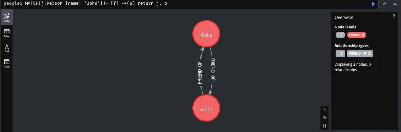
A very exotic variant of NoSQL databases are graph databases, which represent data as graphs. This storage format allows for the efficient storage of information according to relationships. Such relationships can be links between websites or a person’s representation on social media. Even the complex relationships used in recommendation systems can be represented as graphs. The following figure shows a simple example of a graph database implemented in Java using Neo4j, to illustrate its use case.
Other graph databases include Amazon Neptune and ArangoDB.
Finally, I’d like to introduce time series. Since monitoring has become essential, especially in the context of application operation, data presented as time series has gained in importance. Typical databases that specialize in processing time series are Prometheus and InfluxDB. However, there are also corresponding extensions for classic relational databases. The PostgreSQL database, which has already been mentioned several times, also has a corresponding extension for this use case called TimescaleDB.
Of course, much more could be said about this topic. After all, countless books on databases fill several meters of library shelves. However, this should suffice for an introduction and an overview of the various database systems and NoSQL solutions. With the information from this article, you now have an idea of which database is suitable for your specific use case. We have also seen that relational databases, especially the free and open-source database PostgreSQL with its available extensions, are very versatile. Further topics related to databases include data modeling and security against hacker attacks.
Anyone interested in this somewhat specialized article doesn’t need an explanation of what Docker is and what this virtualization tool is used for. Therefore, this article is primarily aimed at system administrators, DevOps engineers, and cloud developers. For those who aren’t yet completely familiar with the technology, I recommend our Docker course: From Zero to Hero.
In a scenario where we regularly create new Docker images and instantiate various containers, our hard drive is put under considerable strain. Depending on their complexity, images can easily reach several hundred megabytes to gigabytes in size. To prevent creating new images from feeling like downloading a three-minute MP3 with a 56k modem, Docker uses a build cache. However, if there’s an error in the Dockerfile, this build cache can become quite bothersome. Therefore, it’s a good idea to clear the build cache regularly. Old container instances that are no longer in use can also lead to strange errors. So, how do you keep your Docker environment clean?
While docker rm <container-nane> and docker rmi <image-id> will certainly get you quite far, in build environments like Jenkins or server clusters, this strategy can become a time-consuming and tedious task. But first, let’s get an overview of the overall situation. The command docker system df will help us with this.
Before I delve into the details, one important note: The commands presented are very efficient and will irrevocably delete the corresponding areas. Therefore, only use these commands in a test environment before using them on production systems. Furthermore, I’ve found it helpful to also version control the commands for instantiating containers in your text file.
The most obvious step in a Docker system cleanup is deleting unused containers. Specifically, this means that the delete command permanently removes all instances of Docker containers that are not running (i.e., not active). If you want to perform a clean slate on a Jenkins build node before deployment, you can first terminate all containers running on the machine with a single command.
The -f parameter suppresses the confirmation prompt, making it ideal for automated scripts. Deleting containers frees up relatively little disk space. The main resource drain comes from downloaded images, which can also be removed with a single command. However, before images can be deleted, it must first be ensured that they are not in use by any containers (even inactive ones). Removing unused containers offers another practical advantage: it releases ports blocked by containers. A port in a host environment can only be bound to a container once, which can quickly lead to error messages. Therefore, we extend our script to include the option to delete all Docker images not currently used by containers.
Another consequence of our efforts concerns Docker layers. For performance reasons, especially in CI environments, you should avoid using them. Docker volumes, on the other hand, are less problematic. When you remove the volumes, only the references in Docker are deleted. The folders and files linked to the containers remain unaffected. The -a parameter deletes all Docker volumes.
docker volume prune -a -f
Another area affected by our cleanup efforts is the build cache. Especially if you’re experimenting with creating new Dockerfiles, it can be very useful to manually clear the cache from time to time. This prevents incorrectly created layers from persisting in the builds and causing unusual errors later in the instantiated container. The corresponding command is:
docker buildx prune -f
The most radical option is to release all unused resources. There is also an explicit shell command for this.
docker volume prune -a -f
We can, of course, also use the commands just presented for CI build environments like Jenkins or GitLab CI. However, this might not necessarily lead to the desired result. A proven approach for Continuous Integration/Continuous Deployment is to set up your own Docker registry where you can deploy your self-built images. This approach provides a good backup and caching system for the Docker images used. Once correctly created, images can be conveniently deployed to different server instances via the local network without having to constantly rebuild them locally. This leads to a proven approach of using a build node specifically optimized for Docker images/containers to optimally test the created images before use. Even on cloud instances like Azure and AWS, you should prioritize good performance and resource efficiency. Costs can quickly escalate and seriously disrupt a stable project.
In this article, we have seen that in-depth knowledge of the tools used offers several opportunities for cost savings. The motto “We do it because we can” is particularly unhelpful in a commercial environment and can quickly degenerate into an expensive waste of resources.
Working with mass storage devices such as hard disks (HDDs), solid-state drives (SSDs), USB drives, memory cards, or network-attached storage devices (NAS) isn’t as difficult under Linux as many people believe. You just have to be able to let go of old habits you’ve developed under Windows. In this compact course, you’ll learn everything you need to master potential problems on Linux desktops and servers.
Before we dive into the topic in depth, a few important facts about the hardware itself. The basic principle here is: Buy cheap, buy twice. The problem isn’t even the device itself that needs replacing, but rather the potentially lost data and the effort of setting everything up again. I’ve had this experience especially with SSDs and memory cards, where it’s quite possible that you’ve been tricked by a fake product and the promised storage space isn’t available, even though the operating system displays full capacity. We’ll discuss how to handle such situations a little later, though.
Another important consideration is continuous operation. Most storage media are not designed to be switched on and used 24 hours a day, 7 days a week. Hard drives and SSDs designed for laptops quickly fail under constant load. Therefore, for continuous operation, as is the case with NAS systems, you should specifically look for such specialized devices. Western Digital, for example, has various product lines. The Red line is designed for continuous operation, as is the case with servers and NAS. It is important to note that the data transfer speed of storage media is generally somewhat lower in exchange for an increased lifespan. But don’t worry, we won’t get lost in all the details that could be said about hardware, and will leave it at that to move on to the next point.
A significant difference between Linux and Windows is the file system, the mechanism by which the operating system organizes access to information. Windows uses NTFS as its file system, while USB sticks and memory cards are often formatted in FAT. The difference is that NTFS can store files larger than 4 GB. FAT is preferred by device manufacturers for navigation systems or car radios due to its stability. Under Linux, the ext3 or ext4 file systems are primarily found. Of course, there are many other specialized formats, which we won’t discuss here. The major difference between Linux and Windows file systems is the security concept. While NTFS has no mechanism to control the creation, opening, or execution of files and directories, this is a fundamental concept for ext3 and ext4.
Storage devices formatted in NTFS or FAT can be easily connected to Linux computers, and their contents can be read. To avoid any risk of data loss when writing to network storage, which is often formatted as NTFS for compatibility reasons, the SAMBA protocol is used. Samba is usually already part of many Linux distributions and can be installed in just a few moments. No special configuration of the service is required.
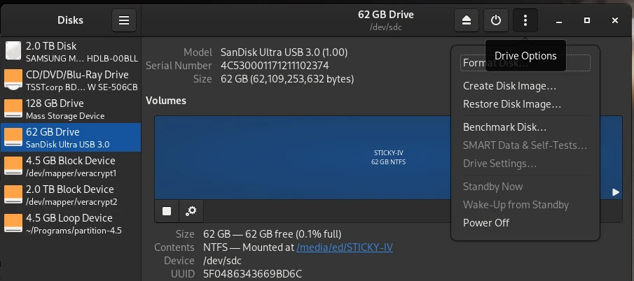
Now that we’ve learned what a file system is and what it’s used for, the question arises: how to format external storage in Linux? The two graphical programs Disks and Gparted are a good combination for this. Disks is a bit more versatile and allows you to create bootable USB sticks, which you can then use to install computers. Gparted is more suitable for extending existing partitions on hard drives or SSDs or for repairing broken partitions.
Before you read on and perhaps try to replicate one or two of these tips, it’s important that I offer a warning here. Before you try anything with your storage media, first create a backup of your data so you can fall back on it in case of disaster. I also expressly advise you to only attempt scenarios you understand and where you know what you’re doing. I assume no liability for any data loss.
One scenario we occasionally need is the creation of bootable media. Whether it’s a USB flash drive for installing a Windows or Linux operating system, or installing the operating system on an SD card for use on a Raspberry Pi, the process is the same. Before we begin, we need an installation medium, which we can usually download as an ISO from the operating system manufacturer’s website, and a corresponding USB flash drive.
Next, open the Disks program and select the USB drive on which we want to install the ISO file. Then, click the three dots at the top of the window and select Restore Disk Image from the menu that appears. In the dialog that opens, select our ISO file for the Image to Restore input field and click Start Restoring. That’s all you need to do.
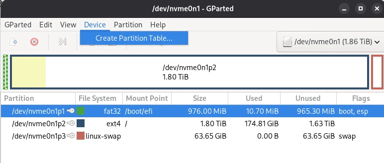
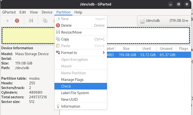
Repairing Partitions and MTF with Gparted
Another scenario you might encounter is that data on a flash drive, for example, is unreadable. If the data itself isn’t corrupted, you might be lucky and be able to solve the problem with GParted. In some cases, (A) the partition table may be corrupted and the operating system simply doesn’t know where to start. Another possibility is (B) the Master File Table (MFT) may be corrupted. The MTF contains information about the memory location in which a file is located. Both problems can be quickly resolved with GParted.
Of course, it’s impossible to cover the many complex aspects of data recovery in a general article.
Now that we know that a hard drive consists of partitions, and these partitions contain a file system, we can now say that all information about a partition and the file system formatted on it is stored in the partition table. To locate all files and directories within a partition, the operating system uses an index, the so-called Master File Table, to search for them. This connection leads us to the next point: the secure deletion of storage media.
Data Shredder – Secure Deletion
When we delete data on a storage medium, only the entry where the file can be found is removed from the MFT. The file therefore still exists and can still be found and read by special programs. Securely deleting files is only possible if we overwrite the free space multiple times. Since we can never know where a file was physically written on a storage medium, we must overwrite the entire free space multiple times after deletion. Specialists recommend three write processes, each with a different pattern, to make recovery impossible even for specialized labs. A Linux program that also sweeps up and deletes “data junk” is BleachBit.
Securely overwriting deleted files is a somewhat lengthy process, depending on the size of the storage device, which is why it should only be done sporadically. However, you should definitely delete old storage devices completely when they are “sorted out” and then either disposed of or passed on to someone else.
Mirroring Entire Hard Drives 1:1 – CloneZilla
Another scenario we may encounter is the need to create a copy of the hard drive. This is relevant when the existing hard drive or SSD for the current computer needs to be replaced with a new one with a higher storage capacity. Windows users often take this opportunity to reinstall their system to keep up with the practice. Those who have been working with Linux for a while appreciate that Linux systems run very stably and the need for a reinstallation only arises sporadically. Therefore, it is a good idea to copy the data from the current hard drive bit by bit to the new drive. This also applies to SSDs, of course, or from HDD to SSD and vice versa. We can accomplish this with the free tool CloneZilla. To do this, we create a bootable USB with CloneZilla and start the computer in the CloneZilla live system. We then connect the new drive to the computer using a SATA/USB adapter and start the data transfer. Before we open up our computer and swap the disks after finishing the installation, we’ll change the boot order in the BIOS and check whether our attempt was successful. Only if the computer boots smoothly from the new disk will we proceed with the physical replacement. This short guide describes the basic procedure; I’ve deliberately omitted a detailed description, as the interface and operation may differ from newer Clonezilla versions.
SWAP – The Paging File in Linux
At this point, we’ll leave the graphical user interface and turn to the command line. We’ll deal with a very special partition that sometimes needs to be expanded. It’s the SWAP file. The SWAP file is what Windows calls the swap file. This means that the operating system writes data that no longer fits into RAM to this file and can then read this data back into RAM more quickly when needed. However, it can happen that this swap file is too small and needs to be expanded. But that’s not rocket science, as we’ll see shortly.
We’ve already discussed quite a bit about handling storage media under Linux. In the second part of this series, we’ll delve deeper into the capabilities of command-line programs and look, for example, at how NAS storage can be permanently mounted in the system. Strategies for identifying defective storage devices will also be the subject of the next part. I hope I’ve piqued your interest and would be delighted if you would share the articles from this blog.
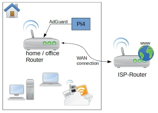
Maybe you have bought you like me an Raspberry Pi4 with 4GB RAM and think about what nice things you could do with it. Since the beginning I got the idea to use it as an lightweight home server. Of course you can easily use a mini computer with more power and obviously more energy consumption too. Not a nice idea for a device is running 24/7. As long you don’t plan to mine your own bitcoins or host a high frequented shop system, a PI device should be sufficient.
I was wanted to increase the network security for my network. For this reason I found the application AdGuard which blocks many spy software from internet services you use on every device is connected to the network where AdGuard is running. Sounds great and is not so difficult to do. Let me share with you my experience.
As first let’s have a look to the overall system and perquisites. After the Router from my Internet Service Provider I connected direct by wire my own Network router an Archer C50. On my Rapsbery PI4 with 4GB RAM run as operation system Ubuntu Linux Server x64 (ARM Architecture). The memory card is a 64 GB ScanDisk Ultra. In the case you need a lot of storage you can connect an external SSD or HDD with an USB 3 – SATA adapter. Be aware that you use a storage is made for permanent usage. Western Digital for example have an label called NAS, which is made for this purpose. If you use standard desktop versions they could get broken quite soon. The PI is connected with the router direct by LAN cable.
The first step you need to do is to install on the Ubuntu the Docker service. this is a simple command: apt-get install docker. if you want to get rid of the sudo you need to add the user to the docker group and restart the docker service. If you want to get a bit more familiar with Docker you can check my video Docker basics in less than 10 minutes.
Before you just copy and past the listing above, you need to change the IP addresses to the ones your network is using. for all the installation, this is the most difficult part. As first the network type we create is macvlan bounded to the network card eth0. eth0 is for the PI4 standard. The name of the network we gonna to create is lan. To get the correct values for subnet, ip-range and gateway you need to connect to your router administration.
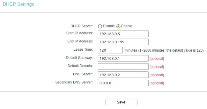
To understand the settings, we need a bit of theory. But don’t worry is not much and not that complicated. Mostly your router is reachable by an IP address similar to 192.168.0.1 – this is a static address and something equal we want to have for AdGuard on the PI. The PI itself is in my case reachable by 192.168.0.12, but this IP we can not use for AdGuard. The plan is to make the AdGuard web interface accessible by the IP 192.168.0.2. OK let’s do it. First we have to switch on our router administration to the point DHCP settings. In the Screenshot you can see my configuration. After you changed your adaptions don’t forget to reboot the router to take affect of the changes.
I configured the dynamic IP range between 192.168.0.5 to 192.168.0.199. This means the first 4 numbers before 192.168.0.5 can be used to connect devices with a static IP. Here we see also the entry for our default gateway. Whit this information we are able to return to our network configuration. the subnet IP is like the gateway just the digits in the last IP segment have to change to a zero. The IP range we had limited to the 192.168.0.4 because is one number less than where we configured where the dynamic IP range started. That’s all we need to know to create our network in Docker on the PI.
Now we need to create in the home directory of our PI the places were AdGuard can store the configuration and the data. This you can do with a simple command in the ssh shell.
The container we create is called adguard and we connect this image to our own created network lan with the IP address 192.168.0.2. Then we have to open a lot of ports AdGuard need to do the job. And finally we connect the two volumes for the configuration and data directory inside of the container. As restart policy we set the container to always, this secure that the service is up again after the server or docker was rebooted.
After the execution of the docker run command you can reach the AdGuard configuration page with your browser under: http://192.168.0.2:3000. Here you can create the primary setup to create a login user and so on. After the first setup you can reach the web interface by http://192.168.0.2.
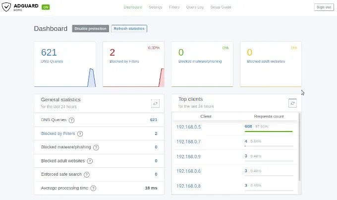
The IP address 192.168.0.2 you need now to past into the field DNS Server for the DHCP settings. Save the entries and restart your router to get all changes working. When the router is up open on your browser any web page from the internet to see that everything is working fine. After this you can login into the AdGuard web console to see if there appearing data on the dashboard. If this is happened then you are don e and your home or office network is protected.
If you think this article was helpful and you like it, you can support my work by sharing this post or leave a like. If you have some suggestions feel free to drop a comment.
For business it’s sometime important to have a central place where employees and clients are able to interact together. NextCloud is a simple and extendable PHP solution with a huge set of features you can host by yourself, to keep full control of your data. A classical Groupware ready for your own cloud.
If you want to install NextCloud on your own server you need as first a well working PHP installation with a HTTP Server like Apache. Also a Database Management System is mandatory. You can chose between MySQL, MariaDB and PostgreSQL servers. The classical way to install and configure all those components takes a lot of time and the maintenance is very difficult. To overcome all this we use a modern approach with the virtualization tool docker.
The system setup is as the following: Ubuntu x64 Server, PostgreSQL Database, pgAdmin DBMS Management and NextCloud.
If you have any question feel free to leave a comment. May you need help to install and operate your own NextCloud installation secure, don’t hesitate to contact us by the contact form. In the case you like the video level a thumbs up and share it.
[EN] We use cookies to improve your experience on our site. By using our site, you consent to cookies.
[DE] Wir verwenden Cookies, um Ihre Erfahrungen auf unserer Website zu verbessern. Durch die Nutzung unserer Website stimmen Sie Cookies zu.
This website uses cookies
Websites store cookies to enhance functionality and personalise your experience. You can manage your preferences, but blocking some cookies may impact site performance and services.
Essential cookies enable basic functions and are necessary for the proper function of the website.
Name
Description
Duration
Cookie Preferences
This cookie is used to store the user's cookie consent preferences.
30 days
These cookies are needed for adding comments on this website.
Name
Description
Duration
comment_author
Used to track the user across multiple sessions.
Session
comment_author_email
Used to track the user across multiple sessions.
Session
comment_author_url
Used to track the user across multiple sessions.
Session
These cookies are used for managing login functionality on this website.
Name
Description
Duration
wordpress_logged_in
Used to store logged-in users.
Persistent
wordpress_sec
Used to track the user across multiple sessions.
15 days
wordpress_test_cookie
Used to determine if cookies are enabled.
Session
Statistics cookies collect information anonymously. This information helps us understand how visitors use our website.
Matomo is an open-source web analytics platform that provides detailed insights into website traffic and user behavior.